Text archives Help

---

This is from a recent offline discussion with Kristen about the best way to remove the dependency to Qt in the currently experimental new Spline Tool.


Currently, I'm using the LGPL library Qwt to compute the spline coefficients and sample the spline. But this library has a dependency to Qt, something we would like to eliminate.

The current Spline Tool computation is done to mimic the results from Matlab's function CSCVN().


There are two possible solutions on the table right now:

1) Write a derivative work of Qwt to remove the dependency to Qt

2) As Kristen has pointed out:

"Another alternative would be to use the spline computation
implemented in src/Dataflow/Modules/Fields/GeneratePlanarElectrode.cc
and src/Dataflow/Modules/Fields/GenerateWireElectrode.cc that is
coded to behave similarly to Matlab's spline computation interp1."


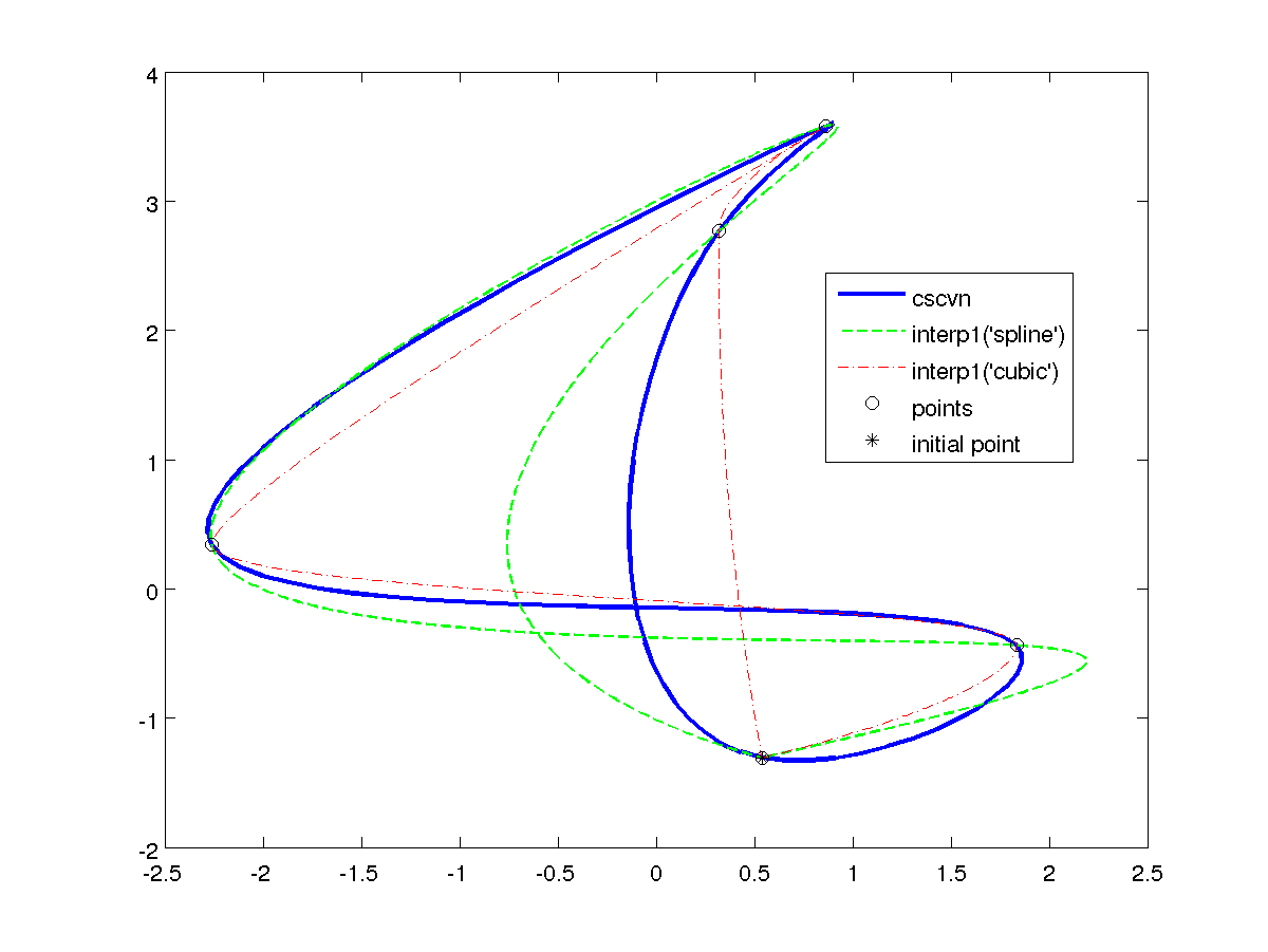
I have checked 2), and it doesn't seem feasible, because the coefficients computed by cscvn and interp1 are different. That is, they compute different splines even if both use the same knot vector. I suppose this have to be because of different end-conditions.

To illustrate this, I have attached a figure comparing the interpolation produced by cscv() to the interpolation of interp1() using cubic and Hermite polynomials.

Also, attached is the Matlab script used to generate it.

Best regards,

Ramon.

--
Dr. Ramón Casero Cañas

Computational Biology, Computing Laboratory
University of Oxford
Wolfson Building, Parks Rd
Oxford OX1 3QD

tlf     +44 (0) 1865 610807
web     http://web.comlab.ox.ac.uk/people/Ramon.CaseroCanas
photos  http://www.flickr.com/photos/rcasero/

% equivalence_between_cscvn_interp1.m
%
% Study the equivalence between the cubic splines computed by Matlab
% functions CSCVN() and INTERP1(). Result: They aren't equivalent.

DOCDIR='/home/ramc/secure_data/comlab/ramc/rcasero/doc/cardio3d-atlas-notes/trunk';

% generate some random points in 2D
x0 = randn(5, 2);

% make them circular
x = x0( [ 1:end 1 ], : );

%% CSCVN

% cubic spline interpolation with cscvn
pp1 = cscvn( x' );

%% INTERP1

% compute breaks using Lee's scheme (same formula as CSCVN)
t = cumsum(sqrt(sum(diff( x ).^2, 2 )));
t = sum((diff(x).^2).');
t = cumsum([0,t.^(1/4)]);

% cubic spline interpolation of each component
pp2x = interp1( t, x( :, 1 ), 'spline', 'pp' );
pp2y = interp1( t, x( :, 2 ), 'spline', 'pp' );

% sample spline points
xy2 = [ ...
    ppval( pp2x, linspace( pp1.breaks( 1 ), pp1.breaks( end ), 1000 ) )', ...
    ppval( pp2y, linspace( pp1.breaks( 1 ), pp1.breaks( end ), 1000 ) )' ];

% Hermite polynomials spline interpolation of each component
pp3x = interp1( t, x( :, 1 ), 'cubic', 'pp' );
pp3y = interp1( t, x( :, 2 ), 'cubic', 'pp' );

% sample spline points
xy3 = [ ...
    ppval( pp3x, linspace( pp1.breaks( 1 ), pp1.breaks( end ), 1000 ) )', ...
    ppval( pp3y, linspace( pp1.breaks( 1 ), pp1.breaks( end ), 1000 ) )' ];

% plot sampled point on top of previous spline
hold off
fnplt(pp1)
hold on
plot( xy2( :, 1 ), xy2( :, 2 ), 'g--', 'LineWidth', 1 )
plot( xy3( :, 1 ), xy3( :, 2 ), 'r-.' )
plot(x(:,1), x(:,2), 'ko')
plot(x(1,1), x(1,2), 'k*')
legend('cscvn', 'interp1(''spline'')', 'interp1(''cubic'')', 'points', 'initial point')

% save plot
saveas( gca, [ DOCDIR '/figures/no-equivalence-between-cscvn-interp1.png' ], 'png' )

---

• [Seg3D] computing the spline in the Spline Tool, Ramón Casero Cañas, 12/10/2009
  • [Seg3D] Re: computing the spline in the Spline Tool, Dana Brooks, 12/10/2009
    • [Seg3D] Re: Re: computing the spline in the Spline Tool, Ramón Casero Cañas, 12/10/2009

---

Archive powered by MHonArc 2.6.16.